salientDIF <- function(m1, s1, m2, s2, threshold = 0.33) {

  # Calculate the mean of the difference D = x2 - x1
  m_D <- m2 - m1

  # Calculate the standard deviation of the difference D = x2 - x1
  s_D <- abs(s2 - s1)

  # Calculate the Z-scores for the positive and negative thresholds
  Z_positive <- (threshold - m_D) / s_D
  Z_negative <- (-threshold - m_D) / s_D

  # Calculate the probability that D is outside the range (-threshold, threshold)
  probability <- pnorm(Z_negative) + (1 - pnorm(Z_positive))

  # Return the calculated probability
  return(probability)
}salientDIF
Introduction
This document provides a detailed explanation of the function salientDIF, which returns a conservative estimate of the probability that a randomly selected member of a (sub-) population (e.g., the subpopulation from which the observed focal group was sampled) has a value for a DIF-adjusted latent trait \(\theta_2 \sim N(m_2, s_2^2)\) (where \(m_2\) is a mean under DIF-adjustment, and \(s_2^2\) is a variance under DIF adjustment) that exceeds \(\text{threshold}\), and where the DIF-naive (i.e., not adjusted for DIF) distribution of ability is \(\theta_1 \sim N(m_1, s_1^2)\). The calculation assumes that \(\theta_1\) and \(\theta_2\) are linearly related and normally distributed. The threshold value defaults to 0.33.
The result approximates the result of estimating factor scores in a DIF-naive model and a DIF-adjusted model computing their difference, and finding the sample proportion with differences in factor scores exceeding the specified threshold. To get the estimate for the total sample, the result should be obtained using means and variances under DIF-naive and DIF-adjusted models for reference and focal groups, and weighted according to subgroup sample size. The result in observed data will be more similar from the result of the salientDIF procedure as the discrete number of latent trait levels, and there differences, increases (i.e., with increasing number of items and increasing number of response categories).
Problem setup
Assume we have two normally distributed variables:
- \(\theta_1 \sim N(m_1, s_1^2)\)
- \(\theta_2 \sim N(m_2, s_2^2)\)
The goal is to calculate the probability that the absolute difference \(|\theta_2 - \theta_1|\) exceeds some \(\text{threshold}\). In other words, what is the expected proportion of a population subgroup that have a large (0.33 population standard deviation units, assuming \(\theta\) is N(0,1) in the population) difference in estimated latent trait level estimated under two different conditions (DIF naive, DIF adjusted). The means and variances can be obtained from model output: for example, by using the TECH4 output from Mplus.
Calculation
Distribution of the Difference
The difference \(D = \theta_2 - \theta_1\) has a mean and variance as follows:
\[ m_D = m_2 - m_1 \] \[ s_D^2 = s_2^2 + s_1^2 - 2\rho s_2 s_1 \] But, if we assume that the correlation between the latent triat estimates under the two generation methods (\(\rho\)) is 1.0, then we can approximate the standard deviation of the difference as:
\[ s_D = |s_2 - s_1| \] This simplification, under the assumption that \(\rho=1\), is obtained with:
\[ \begin{align*} s_D^2 &= s_2^2 + s_1^2 - 2\rho s_2 s_1 \\ s_D^2 &= s_2^2 + s_1^2 - 2 s_2 s_1 \\ s_D^2 &= \left(s_2 - s_1\right)^2 \\ s_D &= \sqrt{\left(s_2 - s_1\right)^2} \\ s_D &= |s_2-s_1| \end{align*} \]
The assumption that \(\rho\), is the correlation of the two latent traits estimated under two different models, is 1.0 is difficult to verify empirically, and may not necessarily be the same as the correlation between two latent trait estimates.1 Under the assumption that \(\rho=1\), which means that the two latent variables may differ in their scaling but would return the same ordering of participants within a subgroup. The assumption that \(\rho \approx 1\) is less reasonable as the number of items with differential factor loadings increases, but reasonable if the DIF was primarily in item difficulty or location parameters. If we assume \(\rho=1\) is overly optimistic, then using \(s_D=|s_2-s_1|\) is an under-estimate of the standard deviation of the difference in factor scores, and the resulting proportion having a difference exceeding the threshold is a conservative (or biased low) estimate.
Z-Score calculation
Given a default \(\text{Threshold} = 0.33\) or any other threshold of interest, we convert the \(\text{Threshold}\) to a z-score relative to the distribution of differences within the focal group:
\[ Z_{\text{positive}} = \frac{\text{Threshold} - m_D}{s_D} \]
\[ Z_{\text{negative}} = \frac{-\text{Threshold} - m_D}{s_D} \]
Probability calculation
The probability that \(D\) is outside the range \((- \text{Threshold}, \text{Threshold})\) is:
\[ P(|D| > \text{Threshold}) = P(D < -\text{Threshold}) + P(D > \text{Threshold}) \]
Using the standard normal distribution CDF, we get:
\[ P(D < -\text{Threshold}) = \Phi(Z_{\text{negative}}) \]
\[ P(D > \text{Threshold}) = 1 - \Phi(Z_{\text{positive}}) \]
So the final probability is:
\[ \text{Probability} = \Phi(Z_{\text{negative}}) + (1 - \Phi(Z_{\text{positive}}) \]
R Function Implementation
Here is the R function salientDIF that performs this calculation:
Demonstration
We will demonstrate the function salientDIF with an example where the means and standard deviations of the two distributions are given as follows:
- \(m_1 = 0.8\)
- \(s_1 = 1\)
- \(m_2 = 0.6\)
- \(s_2 = 1.1\)
Default threshold
# Define the means and standard deviations of the two distributions
m1 <- 0.8  # Mean of θ1
s1 <- 1   # Standard deviation of θ1
m2 <- 0.6  # Mean of θ2
s2 <- 1.1   # Standard deviation of θ2

# Call the function to calculate the probability with the default Pthreshold
probability_default <- salientDIF(m1, s1, m2, s2)
print(probability_default)
[1] 0.09680054Custom threshold
# Define a custom Pthreshold value
threshold <- 0.2

# Call the function to calculate the probability with a specified Pthreshold
probability_custom <- salientDIF(m1, s1, m2, s2, threshold)
print(probability_custom)
[1] 0.5000317Demonstration
Thissen, Steinberg, & Wainer (1993, p71) provide an example data set. They describe the data:
The items we use in our introductory illustrations were included in a conventional orally administered spelling test, with data obtained from 659 undergraduates at the University of Kansas. The reference for this analysis included male students (N = 285) and the focal group is made up of the female students (N = 374). The original test comprised 100 words, but only 4 have been selected for use here. The four words to be spelled are infidelity, panoramic, succumb, and girder. These four items were selected because preliminary analyses suggested that they have very nearly discrimination parameters; this is convenient for purposes of illustration. The data were free-response, so there is no guessing to be considered. The words infidelity, panoramic, and succumb were selected to comprise an “anchor” (a set of items believed to involve no DIF) with information over a range of the \(\theta\)-continuum. The word girder is the studied item; it was selected because it shows substantial differential difficulty for the two groups in these data.
The data were extracted from Thissen et al’s chapter and presented in Table 1 below.
Table 1. Pvalues (proportion correct) for spelling items among women (N = 374) and men (N = 285), from Thissen et al (1993).
Word | Women | Men |
|---|---|---|
girder | 0.46 | 0.63 |
infidelity | 0.82 | 0.75 |
panoramic | 0.61 | 0.64 |
succumb | 0.29 | 0.32 |
DIF-naive model using Mplus
The first step is to estimate a DIF-naive model, or a baseline model. Since I have a studied item and a set of anchor items, I will use a constrained baseline approach to DIF detection (Yoon & Millsap, 2007) and a multiple-group confirmatory factor analysis with categorical dependent variables approach. I will use Mplus (Muthén & Muthén, Los Angeles CA) via Halquist’s (2011) MplusAutomation package in R.
Although Thissen et al (1993) treated men as the referent group and women as the focal group, my habit is to use the larger of the subgroups as the reference group, which is women. This is communicated to Mplus by providing a grouping variable sex where the lower numerical value is assigned to the group I would like to use as the reference group (women)
summarytools::freq(spelling_expanded$sex)Frequencies
spelling_expanded$sex
Type: Numeric
| Freq | % Valid | % Valid Cum. | % Total | % Total Cum. | |
|---|---|---|---|---|---|
| 1 | 374 | 56.75 | 56.75 | 56.75 | 56.75 |
| 2 | 285 | 43.25 | 100.00 | 43.25 | 100.00 |
| 0 | 0.00 | 100.00 | |||
| Total | 659 | 100.00 | 100.00 | 100.00 | 100.00 |
I’m going to use the WLSMV estimator with theta parameterization, as it is one of three scalings of Mplus parameter estimates that is consistent with the two parameter logistic (2PL) model typically used in IRT. I’m going to save the results as an H5 object, and the factor scores, and request the TECH4 output. The TECH4 output will provide model-estimated means and covariance matrices for the latent variables.
model1   <- "f by infidelity* panoramic succumb (l1-l3);
             f by girder (l4);
             f@1 ;
             [infidelity$1] (t1) ;
             [panoramic$1] (t2) ;
             [succumb$1] (t3) ;
             [girder$1] (t4) ;
             infidelity@1 panoramic@1 succumb@1 girder@1 ;
             MODEL MEN: F*;"
savedata1<- "H5RESULTS = model1.h5;
             SAVE = FSCORES;
             FILE=fscoresmodel1.dat;"

# Run Mplus with mplusModeler, as a function taking model and savedata as input
doit <- function(model,savedata) {
  MplusAutomation::mplusModeler(
     MplusAutomation::mplusObject(
       rdata    = spelling_expanded ,
       VARIABLE = "USEVARIABLES = infidelity panoramic succumb girder sex;
                   CATEGORICAL = infidelity panoramic succumb girder ;
                   GROUPING = sex(1 = women 2 = men);" ,
       ANALYSIS = "ESTIMATOR = WLSMV; PARAMETERIZATION = THETA;"  ,
       OUTPUT   = "TECH4;" ,
       MODEL    = model ,
       SAVEDATA = savedata
     ),
     "girder.dat",
     run = TRUE)
}

# run the model
model1 <- doit(model1, savedata1)
<simpleError in length(covcoverageSubsections) == 0 || is.na(covcoverageSubsections): 'length = 2' in coercion to 'logical(1)'>file.remove("model1.out")[1] TRUEfile.copy("girder.out", "model1.out")[1] TRUE# show a table of results
results1 <- MplusAutomation::readModels("model1.out")<simpleError in length(covcoverageSubsections) == 0 || is.na(covcoverageSubsections): 'length = 2' in coercion to 'logical(1)'>texreg::screenreg(results1, single.row=TRUE,
custom.model.names = c("Men","Women"),
stars = numeric(0),
groups=list("Measurement slopes" = 1:4,
"Means" = 5:5,
"Thresholds" = 6:9,
"Variances" = 10:10,
"Residual variances" = 11:14))
========================================================
                              Men           Women
--------------------------------------------------------
Measurement slopes
     INFIDELITY<-F             0.52 (0.11)   0.52 (0.11)
     PANORAMIC<-F              0.70 (0.13)   0.70 (0.13)
     SUCCUMB<-F                0.65 (0.12)   0.65 (0.12)
     GIRDER<-F                 0.83 (0.16)   0.83 (0.16)
Means
     F<-Means                  0.25 (0.13)   0.00 (0.00)
Thresholds
     INFIDELI$1<-Thresholds   -0.87 (0.08)  -0.87 (0.08)
     PANORAMI$1<-Thresholds   -0.33 (0.07)  -0.33 (0.07)
     SUCCUMB$1<-Thresholds     0.70 (0.08)   0.70 (0.08)
     GIRDER$1<-Thresholds     -0.01 (0.08)  -0.01 (0.08)
Variances
     F<->F                     1.51 (0.42)   1.00 (0.00)
Residual variances
     INFIDELITY<->INFIDELITY   1.00 (0.00)   1.00 (0.00)
     PANORAMIC<->PANORAMIC     1.00 (0.00)   1.00 (0.00)
     SUCCUMB<->SUCCUMB         1.00 (0.00)   1.00 (0.00)
     GIRDER<->GIRDER           1.00 (0.00)   1.00 (0.00)
========================================================summary(results1)Estimated using WLSMV
Number of obs: 659, number of (free) parameters: 10
Model: Chi2(df = 10) = 27.426, p = 0.0022
Baseline model: Chi2(df = 12) = 198.362, p = 0
Fit Indices:
CFI = 0.906, TLI = 0.888, SRMR = 0.051
RMSEA = 0.073, 90% CI [0.041, 0.106], p < .05 = 0.111
AIC = NA, BIC = NA The parameter results show measurement slopes that are (i) equal across sex groups (by design) and (ii) on the same scale as 2PL \(a\)-parameters (discrimination) because we are using WLSMV/theta. The thresholds are also equal across group as intended. The thresholds divided by the measurement slopes gives the 2PL \(b\)-parameters (difficulty). The latent variable means and variances are different, and constrined to N(0,1) in women and freely estimated in men. Men have a higher mean spelling ability and greater variance in spelling ability. The item residual variances are fixed to 1 in both groups. With binary items residual variances and differences in them across group are not seperately identified from differences in the measurement slopes. This model has some issues with model fit (CFI is too low, target is 0.95 or higher) and RMSEA is too high (target is less than .06). The SRMR is decent (target is less than 0.08).
The mean and variance of the latent factor F in the two groups can be obtained from the parameter estimates in this model because there are no covariates. These statistics can also be obtained from TECH4, which is a more general tool as it will work when there are covariates. Unfortunately, neither the output-processing of MplusAutomation nor the H5RESULTS from Mplus contain the TECH4 results, so these quantities must be pulled out “by hand”:
showme.section.lines("model1.out","TECHNICAL 4 OUTPUT",40)TECHNICAL 4 OUTPUT
ESTIMATES DERIVED FROM THE MODEL FOR WOMEN
ESTIMATED MEANS FOR THE LATENT VARIABLES
F
________
0.000
ESTIMATED COVARIANCE MATRIX FOR THE LATENT VARIABLES
F
________
F 1.000
ESTIMATED CORRELATION MATRIX FOR THE LATENT VARIABLES
F
________
F 1.000
ESTIMATES DERIVED FROM THE MODEL FOR MEN
ESTIMATED MEANS FOR THE LATENT VARIABLES
F
________
0.248
ESTIMATED COVARIANCE MATRIX FOR THE LATENT VARIABLES
F
________
F 1.514
DIF-adjusted model using Mplus
Now we’ll free up the cross-group constraints on the girder item.
model2   <- "f by infidelity* panoramic succumb (l1-l3);
             f by girder (l#_4); ! # in label assigns group-specific label
             f@1 ;
             [infidelity$1] (t1) ;
             [panoramic$1] (t2) ;
             [succumb$1] (t3) ;
             [girder$1] (t#_4); ! # in label assigns group-specific label
             infidelity@1 panoramic@1 succumb@1 girder@1 ;
             MODEL MEN: F*;"
savedata2<- "H5RESULTS = model2.h5;
             SAVE = FSCORES;
             FILE=fscoresmodel2.dat;"

# run the model (doit function defined above)
model2 <- doit(model2, savedata2)
<simpleError in length(covcoverageSubsections) == 0 || is.na(covcoverageSubsections): 'length = 2' in coercion to 'logical(1)'>file.remove("model2.out")[1] TRUEfile.copy("girder.out", "model2.out")[1] TRUE# show a table of results
results2 <- MplusAutomation::readModels("model2.out")<simpleError in length(covcoverageSubsections) == 0 || is.na(covcoverageSubsections): 'length = 2' in coercion to 'logical(1)'>texreg::screenreg(results2, single.row=TRUE,
custom.model.names = c("Men","Women"),
stars = numeric(0),
groups=list("Measurement slopes" = 1:4,
"Means" = 5:5,
"Thresholds" = 6:9,
"Variances" = 10:10,
"Residual variances" = 11:14))
========================================================
                              Men           Women
--------------------------------------------------------
Measurement slopes
     INFIDELITY<-F             0.54 (0.12)   0.54 (0.12)
     PANORAMIC<-F              0.69 (0.13)   0.69 (0.13)
     SUCCUMB<-F                0.66 (0.14)   0.66 (0.14)
     GIRDER<-F                 0.66 (0.21)   0.81 (0.21)
Means
     F<-Means                  0.00 (0.14)   0.00 (0.00)
Thresholds
     INFIDELI$1<-Thresholds   -0.94 (0.08)  -0.94 (0.08)
     PANORAMI$1<-Thresholds   -0.40 (0.08)  -0.40 (0.08)
     SUCCUMB$1<-Thresholds     0.64 (0.08)   0.64 (0.08)
     GIRDER$1<-Thresholds     -0.43 (0.12)   0.14 (0.09)
Variances
     F<->F                     1.65 (0.57)   1.00 (0.00)
Residual variances
     INFIDELITY<->INFIDELITY   1.00 (0.00)   1.00 (0.00)
     PANORAMIC<->PANORAMIC     1.00 (0.00)   1.00 (0.00)
     SUCCUMB<->SUCCUMB         1.00 (0.00)   1.00 (0.00)
     GIRDER<->GIRDER           1.00 (0.00)   1.00 (0.00)
========================================================summary(results2)Estimated using WLSMV
Number of obs: 659, number of (free) parameters: 12
Model: Chi2(df = 8) = 11.163, p = 0.1926
Baseline model: Chi2(df = 12) = 198.362, p = 0
Fit Indices:
CFI = 0.983, TLI = 0.975, SRMR = 0.044
RMSEA = 0.035, 90% CI [0, 0.078], p < .05 = 0.665
AIC = NA, BIC = NA Separately modeling the measurement slope and threshold for the girder item erases sex differences in the underlying trait. The model now fits well at conventional levels. The relevant TECH4 output is:
showme.section.lines("model2.out","TECHNICAL 4 OUTPUT",40)TECHNICAL 4 OUTPUT
ESTIMATES DERIVED FROM THE MODEL FOR WOMEN
ESTIMATED MEANS FOR THE LATENT VARIABLES
F
________
0.000
ESTIMATED COVARIANCE MATRIX FOR THE LATENT VARIABLES
F
________
F 1.000
ESTIMATED CORRELATION MATRIX FOR THE LATENT VARIABLES
F
________
F 1.000
ESTIMATES DERIVED FROM THE MODEL FOR MEN
ESTIMATED MEANS FOR THE LATENT VARIABLES
F
________
0.004
ESTIMATED COVARIANCE MATRIX FOR THE LATENT VARIABLES
F
________
F 1.652
Comparing factor score estimates
Let’s compare the estimated factor scores. As the estimator is WLS, these are modal a posteriori factor score estimates.
# read the fscores
# retrieve and merge files with factor scores
# code adapted from factor scores example
m1scores <- read.table("fscoresmodel1.dat", header = FALSE)
m2scores <- read.table("fscoresmodel2.dat", header = FALSE)

# Look at out files to find what the column names should be
colnames(m1scores) <- c("infi", "pano", "succ", "gird", "F", "F_SE", "sex")
colnames(m2scores) <- c("infi", "pano", "succ", "gird", "F", "F_SE", "sex")

# extract the factor scores and place in same data frame
# Select and rename columns
m1scores <- m1scores |> dplyr::select(F, sex) |> dplyr::rename(Fm1 = F)
m2scores <- m2scores |> dplyr::select(F) |> dplyr::rename(Fm2 = F)

# match up rows and compute difference in factor scores
scores <- as.data.frame(c(m1scores,m2scores))
scores$D <- scores$Fm2-scores$Fm1
The correlation of the factor scores without and with DIF adjustment is, in women and men:
corr_women <- cor(scores$Fm1[which(scores$sex==1)],scores$Fm2[which(scores$sex==1)])
corr_men <- cor(scores$Fm1[which(scores$sex==2)],scores$Fm2[which(scores$sex==2)])
print(rbind(corr_women,corr_men))
[,1]
corr_women 0.9998891
corr_men 0.9978973which are pretty close to 1. The standard deviations of the factor scores, and their difference, are:
# Compute standard deviations for women and men and round to 3 decimal places
std_devs <- scores %>%
  group_by(sex) %>%
  summarise(across(c(Fm1, Fm2, D), ~ round(sd(.), 3))) %>%
  pivot_longer(cols = -sex, names_to = "Variable", values_to = "Standard_Deviation") %>%
  pivot_wider(names_from = sex, values_from = Standard_Deviation, names_prefix = "Sex_")

# Rename columns for clarity
std_devs <- std_devs %>%
  rename(`Women SD` = Sex_1, `Men SD` = Sex_2)

# Create flextable
ft <- flextable(std_devs)

# Display flextable
ft
Variable | Women SD | Men SD |
|---|---|---|
Fm1 | 0.654 | 0.856 |
Fm2 | 0.657 | 0.904 |
D | 0.010 | 0.074 |
Here is a table that shows the distribution of differences in factor score estimates for men and women:
Table 2. Observed differences in DIF-naive and DIF-adjusted factor score estimates
# Create a frequency table
freq_table <- scores |>
  mutate(D = round(D,2)) |>
  group_by(sex, D) |>
  summarise(Frequency = n(), .groups = 'drop') |>
  pivot_wider(names_from = sex, values_from = Frequency, names_prefix = "Sex_") |>
  arrange(D)

# Replace NA values with 0 (if any)
freq_table[is.na(freq_table)] <- 0

# Create a flextable
ft <- flextable(freq_table) |>
  set_header_labels(sex = "Sex", D = "Difference", Sex_1 = "Women", Sex_2 = "Men") |>
  theme_vanilla() |>
  autofit()

# Display the flextable in the document
ft
Difference | Women | Men |
|---|---|---|
-0.43 | 0 | 10 |
-0.34 | 0 | 41 |
-0.33 | 0 | 22 |
-0.29 | 0 | 1 |
-0.26 | 0 | 97 |
-0.25 | 0 | 8 |
-0.22 | 0 | 8 |
-0.21 | 0 | 1 |
-0.20 | 0 | 24 |
-0.18 | 0 | 1 |
-0.16 | 0 | 62 |
-0.11 | 0 | 10 |
-0.02 | 25 | 0 |
-0.01 | 36 | 0 |
0.00 | 71 | 0 |
0.01 | 208 | 0 |
0.02 | 12 | 0 |
0.03 | 22 | 0 |
The thing to notice is that there are men who have substantial differences in their latent trait estimate, but women do not have many individuals with large changes in ability estimates. The observed differences in estimated factor scores are also “lumpy”. With 4 items each with 2 categories, there are 2^4 = 16 possible response patterns, and each response pattern will have a specific \(\theta\) estimate, and possible \(\theta\) difference under two different sets of parameters. The point being, this number is finite.
There are 10+41+22 mean with absolute differences greater than 0.33, and since there are 285 men, 0.256 men have what we would consider salient DIF.
Using the salientDIF function
# Tech4 output from model 1
# women
m11 <- 0 # mean, model = 1, sex = 1 (women)
V11 <- 1 # variance, model = 1, sex = 1 (women)
# men
m12 <- 0.248 # mean, model = 1, sex = 2 (men)
V12 <- 1.514 # mean, model = 1, sex = 2 (men)
# Tech4 output from model 2
# women
m21 <- 0 # mean, model = 2, sex = 1 (women)
V21 <- 1 # variance, model = 2, sex = 1 (women)
# men
m22 <- 0.004 # mean, model = 2, sex = 2 (men)
V22 <- 1.652 # mean, model = 2, sex = 2 (men)

threshold <- 0.33
salientDIF_women <- salientDIF(m21,sqrt(V21),m11,sqrt(V11), threshold = threshold)
salientDIF_men   <- salientDIF(m22,sqrt(V22),m12,sqrt(V12), threshold = threshold)

print(rbind(salientDIF_women,salientDIF_men))
[,1]
salientDIF_women 0.00000000
salientDIF_men 0.05846562That looks like a pretty big miss. But it is not a miss: the issue has to do with the “lumpiness” of the observed difference scores. To illustrate this point I will draw a set of curves that show the observed, given the example data set of spelling questions, and salientDIF function implied proportion with salient DIF at different thresholds, ranging from 0.05 to 0.40.
fun1 <- function(threshold) {
   scores |> filter(sex == 2) |> mutate(hit = abs(D) > threshold) |> pull(hit) |> mean()
}
fun2 <- function(threshold) {
  m22 <- 0.004 # mean, model = 2, sex = 2 (men)
  V22 <- 1.652 # mean, model = 2, sex = 2 (men)
  m12 <- 0.248 # mean, model = 1, sex = 2 (men)
  V12 <- 1.514 # mean, model = 1, sex = 2 (men)
  salientDIF(m22,sqrt(V22),m12,sqrt(V12), threshold = threshold)
}
fun1(.33)
[1] 0.2561404fun2(.33)[1] 0.05846562Figure 1. Observed proportion and expected proportion (given salientDIF function results) have a threshold or greater difference in factor score estimates from DIF-adjusted and DIF-naive models as the threshold varies from .05 to .40.
library(ggplot2)
# Generate a sequence of threshold values
threshold_values <- seq(0.05, 0.40, by = 0.01)

data <- data.frame(
  threshold = rep(threshold_values, 2),
  value = c(sapply(threshold_values, fun1), sapply(threshold_values, fun2)),
  fun = rep(c("observed", "salientDIF()"), each = length(threshold_values))
)

# Plot the curves using ggplot2
p <- ggplot(data, aes(x = threshold, y = value, color = fun)) +
  geom_line(linewidth = 1) +
  labs(title = "",
       x = "Threshold for salient DIF",
       y = "Predicted or observed proportion with salient DIF") +
  theme_minimal() +
  theme(legend.position = c(0.125, 0.11),  # Position the legend inside the plot
        legend.title = element_blank())  # Remove the legend title

# Save the plot as a high-DPI PNG file
png_file <- "salientDIF_figure1.png"
ggsave(png_file, plot = p, dpi = 800, width = 6, height = 4)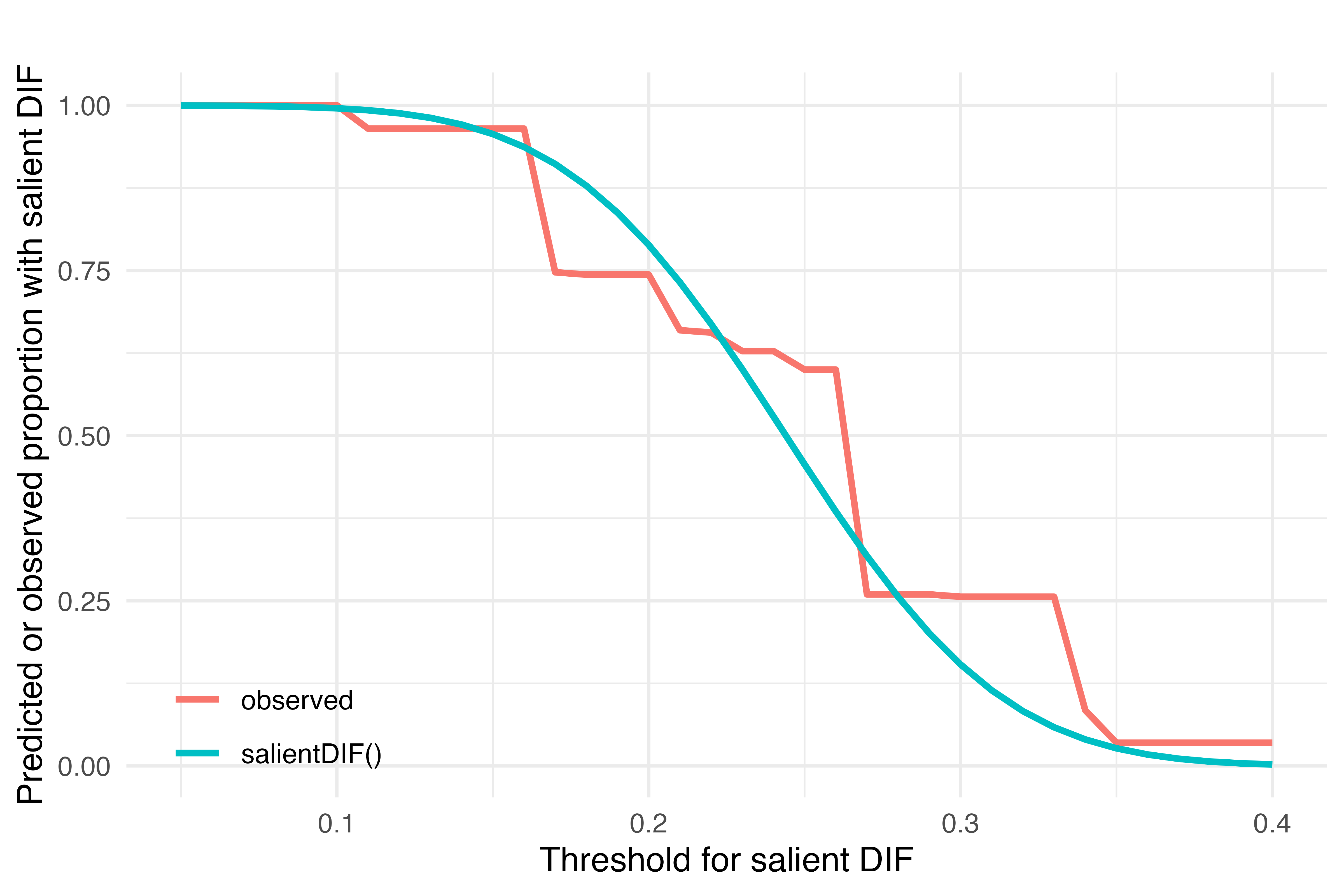
These functions line up very well. However we see that if an analyst had chosen a threshold for salient DIF between about .27 and .34 standard deviation units, the observed proportion of men with salient DIF would have been constant at .25. But the population level results would imply a proportion decreasing from about .25 to .01 across this range. Therefore, the observed proportion with salient DIF is identified as an unreliable reporter of the proportion with DIF that might be expected given the magnitude of differences in the latent trait estimate in a different sample or with different assessment items.
Discussion
The term salient DIF is, to my knowledge, effectively a colloquialism among applied researchers in measurement invariance and differential item functioning detection. In this essay, the term salient DIF is meant to imply DIF that is worth noticing as determined by the impact of the DIF on the overall performance estimate. However, some authors (e.g., Teresi et al, 2022, pp S87-S88) use the term salient DIF when describing item-level DIF (impact typically describes score-level or test -level effects):
DIF saliency was identified by (1) DIF identified after adjustment for multiple comparisons; (2) consistent DIF across methods; (3) high magnitude of DIF; and (4) confirmatory hypotheses consistent with the DIF findings. Three levels of DIF salience were identified and indicated in a table with the following indicators: level 1 is an indication that DIF was detected by IRT-PRO adjusted for multiple comparisons or OLR R2 (McFadden Pseudo R2 criterion ≥0.02, Nagelkerke Pseudo R2 criterion ≥0.02, or Cox-Snell Pseudo R2 criterion ≥0.02) or NCDIF above threshold; level 2 indicates that DIF was detected by IRTPRO or OLR R2 and additionally by NCDIF above threshold; and level 3 indicates that all 3 tests indicated DIF.
To be clear, Teresi et al’s (2022) item-level classification of DIF detection results is not the same kind of DIF saliency addressed in this essay. The meaning intended herein matches more close that suggested by Crane et al (2007)
We introduce here a new approach to determining the scale-level impact of DIF related to each covariate. We calculated the difference between each subject’s score when accounting for DIF and their score when ignoring DIF (the unadjusted score). If DIF makes a negligible difference on scale-level scores, each subject’s difference should be close to zero. If DIF makes a large difference, the value of this difference will be large. We have plotted these differences between scores adjusted for DIF and scores that ignore DIF using box-and-whiskers plots. Previous work has identified differences of 0.33 to 0.50 standard deviation units as the minimally important differences for these scales [42–44].2 If the scale-level impact of DIF is less than the minimally important difference for all subjects, we suggest that DIF related to that covariate is not clinically meaningful for any subject and therefore may be safely ignored. If the scale-level impact of DIF is greater than the minimally important difference for some subjects, we state that the item has relevant (non-ignorable) scale-level differential functioning related to that covariate. Because we used three different criteria
Effect size considerations
There are two aspects of the size of statistics derived from a salientDIF procedure. The first is the threshold used to define salient DIF, and the second is the resulting proportion that is important.
Different authors use different thresholds. Crane et al (2007) suggests 0.33-0.50 standard deviation based on Cella’s work identifying minimally important differences for continuous outcomes in cancer trials. Choi, Gibbons & Crane (2011) use the median standard error of measurement, and argue it is a reasonable threshold when there is no other guidance available. Vonk and colleagues (2022) use a full standard error for the sample (which may be the mean SEM for the sample, as they cite Choi et al (2011) as a reference for that threshold). My rationale for a default threshold of 0.33 is, assuming that the latent trait is distributed normal with mean of zero and standard deviation 1 in the reference group, a value of 0.33 for the standard error of measurement would correspond to a reliability of .89 (a reliability of .9 would be SEM of 0.316). This is also close to a level of precision used as a stopping rule in adaptive testing (Wang, 2019).
The field offers even less insight into what an acceptable proportion would be, or at what fraction of a sample with salient DIF, the detected DIF is no longer ignorable. Choi et al (2011) found 2% of their sample had salient DIF using a median standard deviation (0.2) in their sample, and considered that evidence of ignorable DIF. Vonk and colleagues (2022) found that 7% of their sample had salient DIF (presumably using a mean standard error of measurement) and described that as “considerable” (page 12/17). Therefore somewhere between 2 an 7% falling above an arbitrary threshold is where the DIF impact transitions from “ignorable” to “considerable”.
Clearly more research is needed in interpreting the salientDIF proportion result.
References
Choi, S. W., Gibbons, L. E., & Crane, P. K. (2011). Lordif: An R package for detecting differential item functioning using iterative hybrid ordinal logistic regression/item response theory and Monte Carlo simulations. Journal of statistical software, 39(8), 1.
Crane, P. K., Gibbons, L. E., Narasimhalu, K., Lai, J.-S., & Cella, D. (2007). Rapid detection of differential item functioning in assessments of health-related quality of life: The functional assessment of cancer therapy. Quality of Life Research, 16, 101-114.
Halquist, M. (2011). Mplus Automation. R package version 0.4-2. http://cran.r-project.org/web/packages/Mplusautomation/vignettes/vignette.pdf
Teresi, J. A., Ocepek-Welikson, K., Ramirez, M., Kleinman, M., Wang, C., Weiss, D. J., & Cheville, A. (2022). Examination of the measurement equivalence of the Functional Assessment in Acute Care MCAT (FAMCAT) mobility item bank using differential item functioning analyses. Archives of Physical Medicine and Rehabilitation, 103(5), S84-S107. e138.
Thissen, D., Steinberg, L., & Wainer, H. (1993). Detection of differential item functioning using the parameters of item response models. In P. Holland & H. Wainer (Eds.), Differential item functioning (pp. 67-113). Lawrence Erlbaum Associates, Publishers.
Yoon, M., & Millsap, R. E. (2007). Detecting violations of factorial invariance using data-based specification searches: A Monte Carlo study. Structural Equation Modeling: A Multidisciplinary Journal, 14(3), 435-463.
Vonk, J. M. J., Gross, A. L., Zammit, A. R., Bertola, L., Avila, J. F., Jutten, R. J., Gaynor, L. S., Suemoto, C. K., Kobayashi, L. C., O’Connell, M. E., Elugbadebo, O., Amofa, P. A., Staffaroni, A. M., Arce Renteria, M., Turney, I. C., Jones, R. N., Manly, J. J., Lee, J., & Zahodne, L. B. (2022). Cross-national harmonization of cognitive measures across HRS HCAP (USA) and LASI-DAD (India). PloS one, 17(2), e0264166. https://doi.org/10.1371/journal.pone.0264166
Wang, C., Weiss, D. J., & Shang, Z. (2019). Variable-length stopping rules for multidimensional computerized adaptive testing. Psychometrika, 84(3), 749-771.
Footnotes
probably the best that could be done, in Mplus, is to estimate the two models, separately, using a Bayes estimator and obtaining thousands of estimates for the latent trait per person, treating these as multiply imputed data and estimate the correlation using these multiple imputations. An analytic solution would be better.↩︎
[42.] Cella D, Eton DT, Lai JS, Peterman AH, Merkel DE. Combining anchor and distribution-based methods to derive minimal clinically important differences on the Functional Assessment of Cancer Therapy (FACT) anemia and fatigue scales. J Pain Symptom Manage 2002; 24: 547–561; [43.] Eton DT, Cella D, Yost KJ, et al. A combination of distribution- and anchor-based approaches determined minimally important differences (MIDs) for four endpoints in a breast cancer scale. J Clin Epidemiol 2004; 57: 898–910; [44.] Yost KJ, Sorensen MV, Hahn EA, Glendenning GA, Gnanasakthy A, Cella D. Using multiple anchor- and distribution-based estimates to evaluate clinically meaningful change on the Functional Assessment of Cancer Therapy-Biologic Response Modifiers (FACT-BRM) instrument. Value Health 2005; 8: 117–27.↩︎